Principal component analysis (PCA) is frequently used for analysis of single-cell RNA-seq (scRNA-seq) data. We can use it to reduce the dimensionality of a large matrix with thousands of features (genes) to a smaller matrix with just a few factors (principal components). Since the latest scRNA-seq datasets include millions of cells, there is a need for efficient algorithms. Specifically, we need algorithms that work with sparse matrices instead of dense matrices. Here, we benchmark five implementations of singular value decomposition (SVD) and PCA.
Introduction to PCA and SVD #
For a comprehensive introduction to PCA and how to use it for data analysis, please see:
- Herve Abdi and Lynne J. Williams. Principal component analysis. (27 pages, free PDF)
Compare 5 functions for principal component analysis #
stats::prcomp() from base R.
rsvd::rpca() from the rsvd R package by Ben Erichson.
RSpectra::svds() from the RSpectra R package by Yixuan Qiu.
irlba::prcomp_irlba() and irlba::irlba() From the irlba R package by B. W. Lewis.
install.packages(c("rsvd", "RSpectra", "irlba"))
Load single-cell RNA-seq data #
We use the dataset of epithelial (Epi) cells published in an article by Smillie et al. 2019, which is available for download at SCP259.
a1 <- qread("Smillie2019-Epi-counts.qs")
Let’s count the number of genes (rows) and cells (columns). And let’s see how many entries in the matrix are non-zero:
dim(a1$counts)
## [1] 20028 123006
get_density <- function(x) length(x@x) / x@Dim[1] / x@Dim[2]

get_density(a1$counts)
## [1] 0.07080145
Next, let’s normalize the unique molecular identifier (UMI) counts to log1p counts per million (CPM). We use the median of the number of UMIs per cell as the scaling factor for all cells.
counts_to_cpm <- function(A, norm = median(Matrix::colSums(A))) {
  A@x <- A@x / rep.int(Matrix::colSums(A), diff(A@p))
  A@x <- norm * A@x
  return(A)
}
a1$logcpm <- log1p(counts_to_cpm(a1$counts))
Before we run PCA, let’s filter the set of features (genes) in our dataset. We exclude 37 mitochondrial genes that begin with the string “MT-”, because we’re interested in the variation of other genes. Next, we use loess regression to model the relationship between log10(mean) and log10(sd) for each gene, computed from the raw counts. We select the genes with highest residual variance from that model.
# Exclude MT genes
mito_genes <- rownames(a1$counts)[which(str_detect(rownames(a1$counts), "^MT-"))]

# Fit a model from raw counts that captures log10(sd) ~ log10(mean)
a1$loess <- do_loess(a1$counts, exclude_genes = mito_genes, loess_span = 0.1, min_percent = 0.1)

# Select genes with greatest residual variation
a1$selected_genes <- (
  a1$loess$est %>%
  filter(!is.na(residuals)) %>%
  mutate(selected = residuals > quantile(residuals, 0.85)) %>%
  filter(selected)
)$gene

mat <- a1$logcpm[a1$selected_genes,]
Run PCA or SVD with each function #
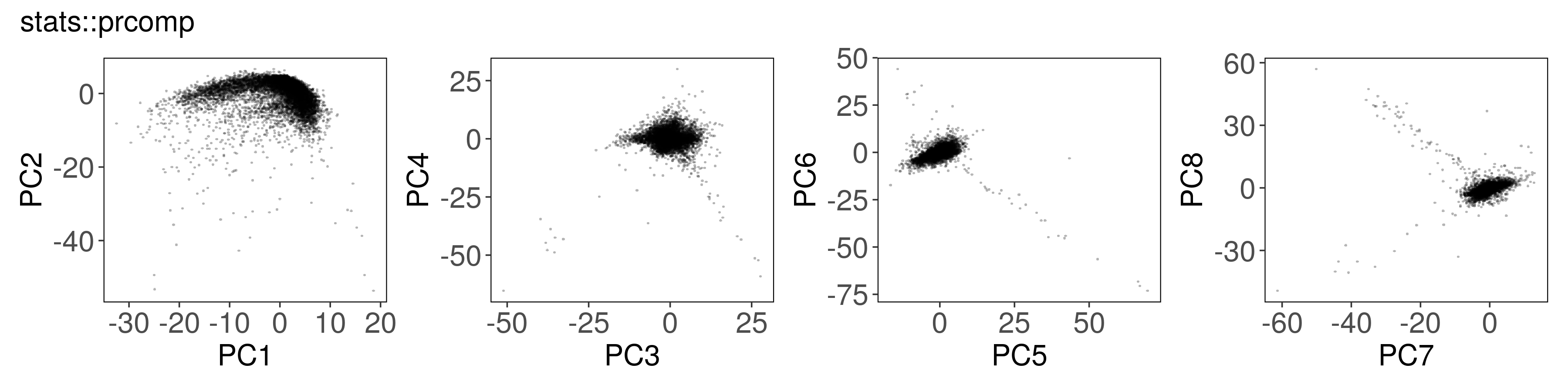
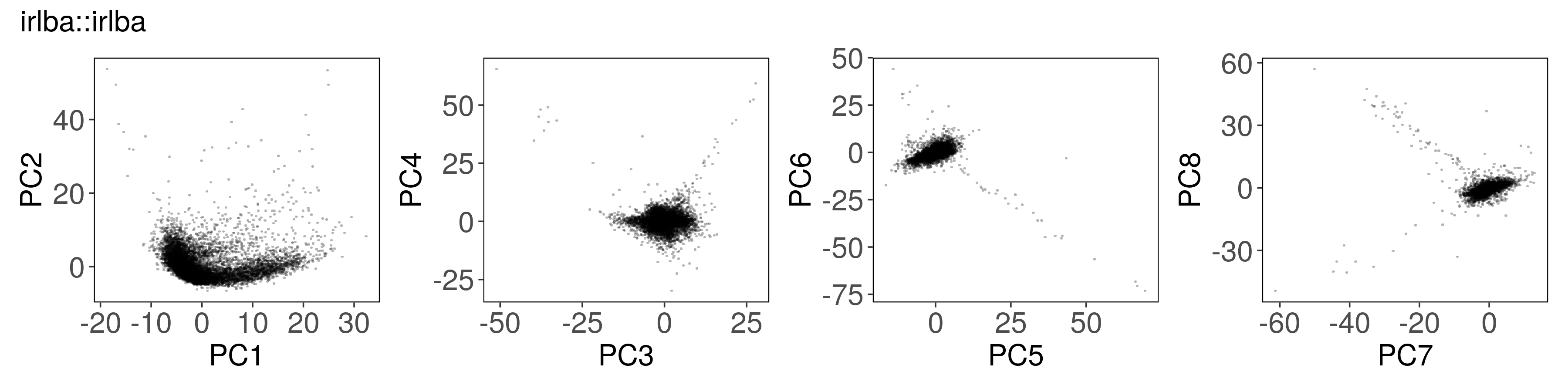
Below, we can see how to run PCA with each function, along with a plot of the
first few factors (e.g., from mat_prcomp$x or mat_svds$x) returned by each
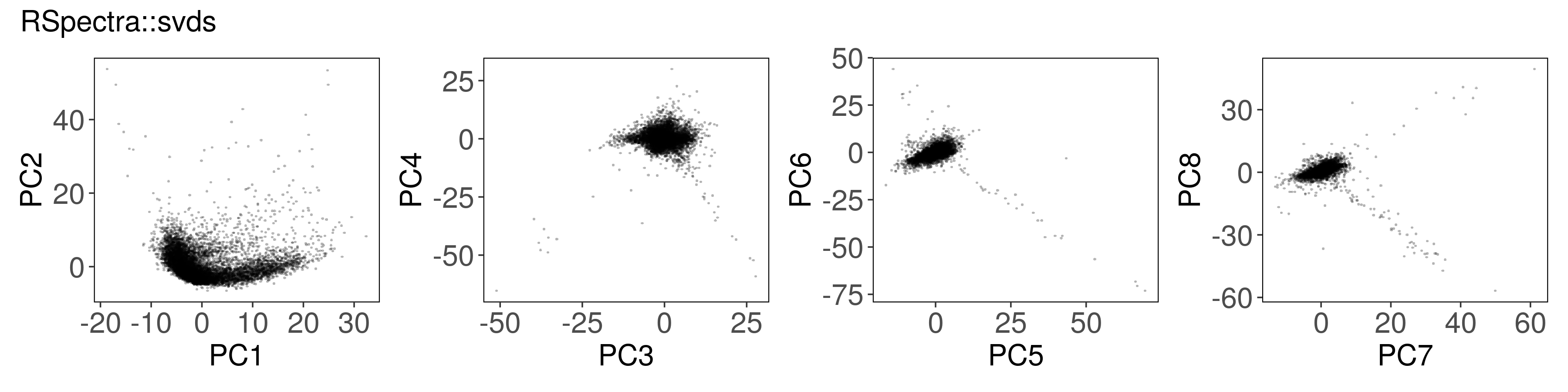
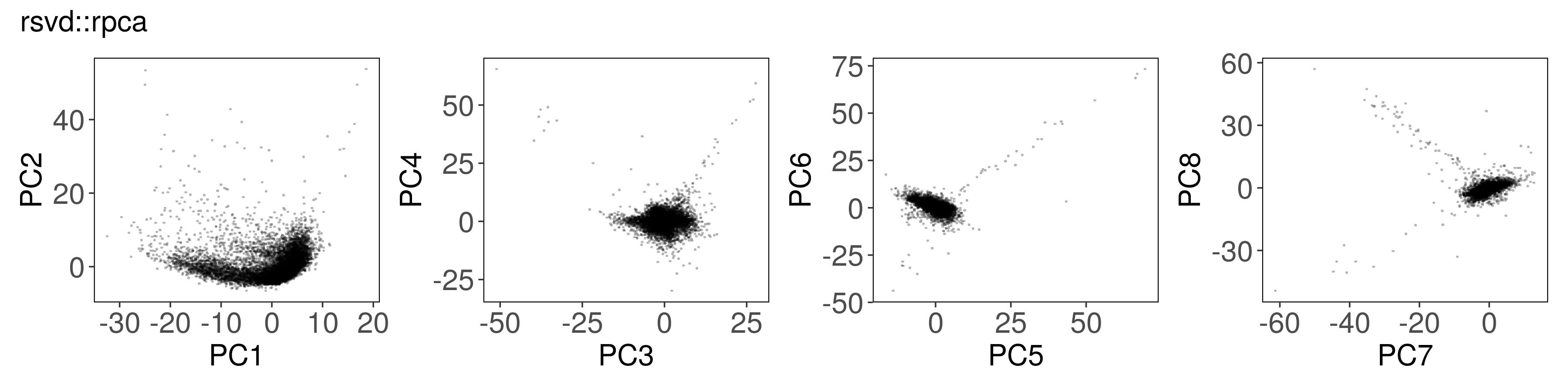
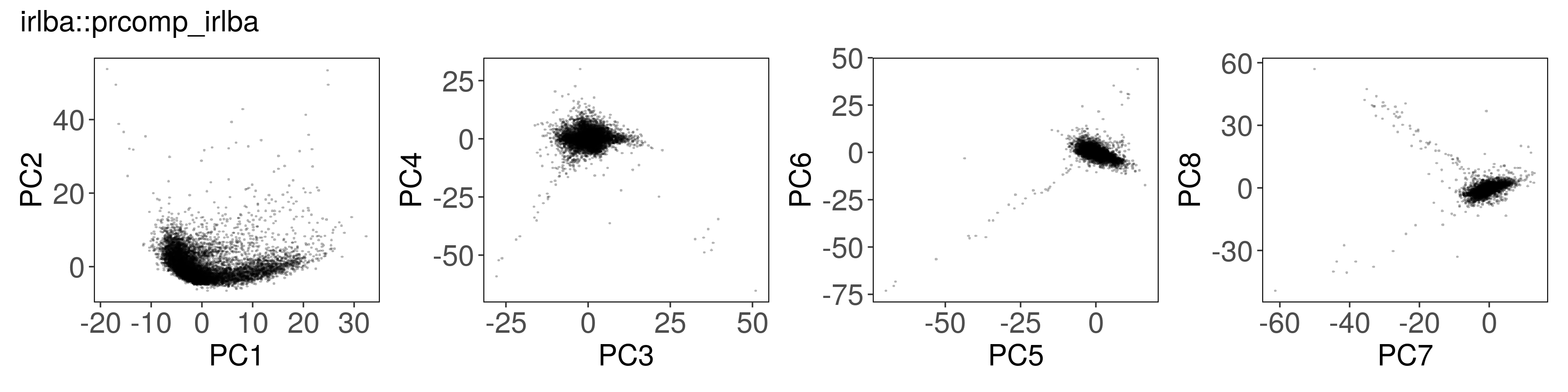
function. The plots look nearly identical, except that the sign is sometimes
flipped. The sign flips are expected and will not affect downstream results.
stats::prcomp() #
mat_prcomp <- prcomp(t(mat), center = TRUE, scale = TRUE, rank. = n_pcs)
Rspectra::svds() #
mat_svds <- RSpectra::svds(
  A    = t(mat),
  k    = n_pcs,
  opts = list(center = TRUE, scale = TRUE)
)
mat_svds$d <- mat_svds$d * sqrt(nrow(mat_svds$u) - 1)
mat_svds$x <- mat_svds$u %*% diag(mat_svds$d)
rsvd::rpca() #
mat_rpca <- rsvd::rpca(
  A      = t(mat),
  k      = n_pcs,# number of dominant principle components to be computed
  center = TRUE, # zero center the variables
  scale  = TRUE, # unit variance the variables
  retx   = TRUE, # return rotated variables
  p      = 20,   # oversampling parameter for rsvd (default p=10)
  q      = n_pcs - 1, # number of additional power iterations for rsvd (default q=1)
  rand   = TRUE  # if (TRUE), the rsvd routine is used, otherwise svd is used
)
irlba::prcomp_irlba() #
mat_irlba <- irlba::prcomp_irlba(
  x      = t(mat),
  n      = n_pcs,
  center = TRUE,
  scale. = TRUE
)
irlba::irlba() #
mat_irlba2 <- irlba::irlba(
  A      = t(mat),
  nv     = n_pcs,
  center = Matrix::rowMeans(mat),
  scale  = proxyC::rowSds(mat)
)
mat_irlba2$x <- mat_irlba2$u %*% diag(mat_irlba2$d)
All of the PCA results are similar to each other #
We expect slight fluctuations in the outputs due to implementation details, but the results should be similar between all of the functions.
The root mean squared error might be a reasonable metric to assess similarity of two vectors:
# Root Mean Squared Error
rmse <- function(x, y) sqrt( sum((x - y) ^ 2) / length(x) )
The factor scores are similar to what we get from stats::prcomp():
rbindlist(lapply(
  list("mat_svds", "mat_rpca", "mat_irlba", "mat_irlba2"),
  function(x) {
    list(
      method = x,
      rmse = rmse( abs( mat_prcomp$x[,1] ), abs( get(x)$x[,1] ) )
    )
  }
)) %>% mutate_if(is.numeric, signif, 2)
##        method    rmse
## 1:   mat_svds 7.6e-09
## 2:   mat_rpca 1.1e-13
## 3:  mat_irlba 2.9e-14
## 4: mat_irlba2 5.7e-14
Suppose the stats::prcomp() output is correct. Are the other outputs
correlated?
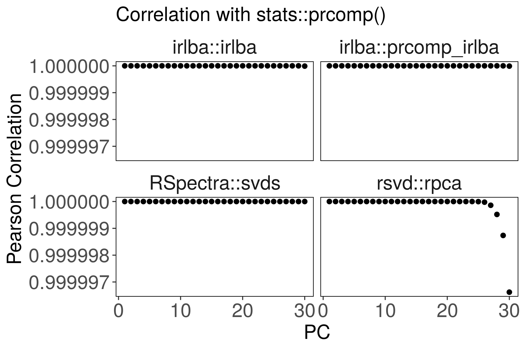
For rsvd::rpca(), the last PCs are slightly less correlated with
stats::prcomp(). We can improve the correlation by increasing p and q
parameters.
Run time and memory usage with increasing number of cells #
The latest scRNA-seq datasets have millions of cells, so it’s important to find methods that can handle large datasets.
We use the bench R package to measure run time and memory usage for each function:
mat <- a1$logcpm[a1$selected_genes,]
dim(mat)
## [1] 2409 123006
mat_meta <- a1$obs[match(colnames(mat), a1$obs$NAME),]
all(mat_meta$NAME == colnames(mat))
## [1] TRUE
# Helper function to take a subset of cells from mat
prep_matrix <- function(n_cells) {
  set.seed(42)
  X <- mat[,sample.int(n = ncol(mat), size = n_cells)]
  if (nrow(X) > ncol(X)) { # If more genes than cells, use fewer genes
    X <- X[1:(ncol(X)/2),]
  }
  X <- X[rowSums(X) > 0,]
  X <- X[,colSums(X) > 0]
  return(X)
}

file_bench <- "pca-benchmark.tsv"
if (file.exists(file_bench)) {

  d <- fread(file_bench)

} else {

  pca_bench <- bench::press(
    n_cells = c(1000, 2000, 4000, 8000, 32000, 64000, 123006),
    {
      X <- prep_matrix(n_cells)
      bench::mark(
        check = FALSE,
        time_unit = 's',
        max_iterations = 5,
        "stats::prcomp()" = {
          prcomp(t(X), center = TRUE, scale = TRUE, rank. = 20)
        },
        "RSpectra::svds()" = {
          retval <- RSpectra::svds(A = t(X), k = 20, opts = list(center = TRUE, scale = TRUE))
          retval$d <- retval$d * sqrt(nrow(retval$u) - 1)
          retval$x <- retval$u %*% diag(retval$d)
          retval
        },
        "irlba::prcomp_irlba()" = {
          irlba::prcomp_irlba(x = t(X), n = 20, center = TRUE, scale. = TRUE)
        },
        "irlba::irlba()" = {
          X_center <- rowMeans(X)
          X_scale <- proxyC::rowSds(X)
          suppressWarnings({
            retval <- irlba::irlba(A = t(X), nv = 20, center = X_center, scale = X_scale)
          })
          retval$x <- retval$u %*% diag(retval$d)
          retval
        },
        "rsvd::rpca()" =  {
          rsvd::rpca(
            A = t(X), k = 20, center = TRUE, scale = TRUE, retx = TRUE,
            p = 10, q = 19, rand = TRUE
          )
        }
      )
    }
  )

  pca_bench$method = attr(pca_bench$expression, "description")
  fwrite(
    x = as_tibble(pca_bench) %>% select(-expression, -result, -memory, -time, -gc),
    file = file_bench,
    sep = "\t"
  )

}
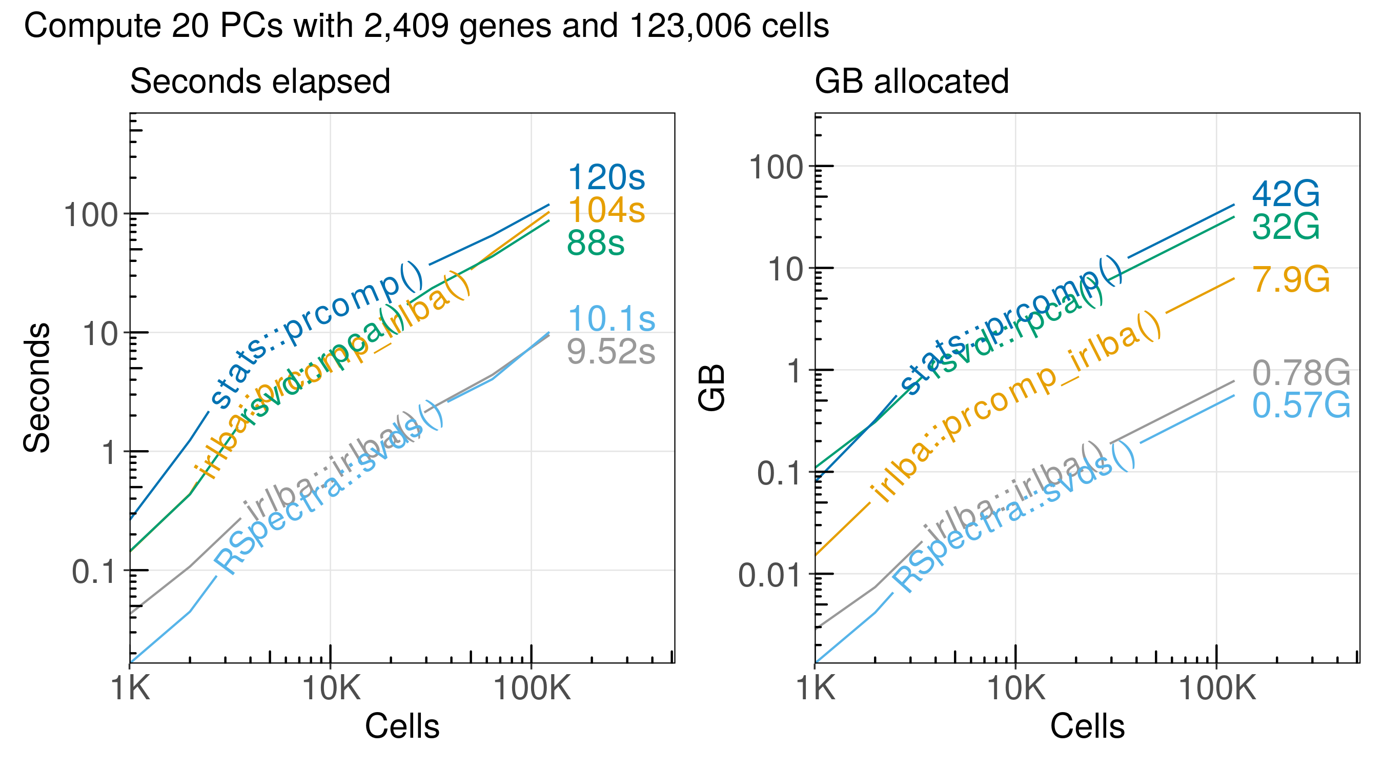
The run time and memory usage of each algorithm increases in proportion to the number of cells we analyze:
Here is a summary of the performance:
| method | n_cells | seconds | gb | cells_per_second | cells_per_gb |
|---|---|---|---|---|---|
| stats::prcomp() | 123,000 | 120.00 | 42.10 | 1,030 | 2,920 |
| irlba::prcomp_irlba() | 123,000 | 104.00 | 7.93 | 1,190 | 15,500 |
| rsvd::rpca() | 123,000 | 88.00 | 31.90 | 1,400 | 3,850 |
| RSpectra::svds() | 123,000 | 10.10 | 0.56 | 12,200 | 218,000 |
| irlba::irlba() | 123,000 | 9.52 | 0.78 | 12,900 | 157,000 |
Conclusions #
The functions RSpectra::svds() and irlba::irlba() are the most efficient
for computing the SVD for a sparse matrix with single-cell RNA-seq data.
The RSpectra::svds() function has the most efficient memory usage, but it is
almost the same as irlba::irlba().
How large is the matrix after manually scaling each gene? #
After scaling, most of the entries in the matrix will no longer be equal to zero. So, the resulting matrix will be represented as a dense matrix instead. We often want to avoid forming the dense matrix in order to avoid using more memory.
How large is the resulting dense matrix?
# Center and scale each row of a sparse matrix.
scale_data <- function(X) {
  X_mean <- Matrix::rowMeans(X)
  X_std <- proxyC::rowSds(X)
  X <- as.matrix(X - X_mean)
  X <- X / X_std
  X[is.na(X)] <- 0
  return(X)
}
# The sparse matrix with logcpm values
size1 <- pryr::object_size(mat)
size1
## 325,439,488 B
# The dense matrix with scaled (mean 0 variance 1) values
size2 <- pryr::object_size(scale_data(mat))
size2
## 2,381,553,440 B
The memory allocation increases 7.3-fold for the dense scaled matrix. Note that irlba and RSpectra manage to effectively scale the data without allocating 2.38 GB of memory!
What is the maximum number of cells we can analyze in R? #
One way to address this question is to check how much memory is allocated for a matrix with different sizes, but with the same density as a real data matrix.
# Density of a real scRNA-seq matrix is usually between 5% and 10%
length(mat@x) / (mat@Dim[1] * mat@Dim[2])
# 0.088

sim <- rsparsematrix(nrow = 2409, ncol = 1e6, density = 0.088)
pryr::object_size(sim)
# 2.55 GB

sim <- rsparsematrix(nrow = 2409, ncol = 2e6, density = 0.088)
pryr::object_size(sim)
# 5.1 GB
It seems that we need about 2.55G of memory per million cells if we keep 2,409 genes per cell.
If we assume 0.088 density and 2409 genes, then we might expect to be able to analyze up to 10 or 11 million cells before we hit the 32 bit limit.
2409 * 11e6 * 0.088 > .Machine$integer.max
## [1] TRUE
It may be more realistic to assume 0.088 density and 20,000 genes. We’ll want to compute statistics for each gene first, and then pass the filtered matrix to downstream functions. That means we will already hit the 32 bit limit when we try to read a counts matrix with 2 million cells and 20,000 genes:
2e4 * 2e6 * 0.088 > .Machine$integer.max
## [1] TRUE
Package versions #
Here are the version numbers of the tested packages at the time of writing:
| version | url | |
|---|---|---|
| RSpectra | 0.16.0 | https://github.com/yixuan/RSpectra |
| rsvd | 1.0.5 | https://github.com/erichson/rSVD |
| irlba | 2.3.5 | https://github.com/bwlewis/irlba |
| Matrix | 1.4.0 | https://CRAN.R-project.org/package=Matrix |
| proxyC | 0.2.4 | https://github.com/koheiw/proxyC |
Related work #
This tutorial explains how to use RSpectra::svds() to get the same results as
stats::prcomp():
This benchmark compares different functions for PCA on large dense matrices:
PCA implementation for sparse matrices in Python:
Session information #
Here are the version numbers for all of the software:
Session info
sessionInfo()
## R version 4.1.0 (2021-05-18)
## Platform: x86_64-pc-linux-gnu (64-bit)
## Running under: Ubuntu 18.04.5 LTS
##
## Matrix products: default
## BLAS:   /usr/lib/x86_64-linux-gnu/openblas/libblas.so.3
## LAPACK: /usr/lib/x86_64-linux-gnu/libopenblasp-r0.2.20.so
##
## locale:
##  [1] LC_CTYPE=en_US.UTF-8       LC_NUMERIC=C
##  [3] LC_TIME=en_US.UTF-8        LC_COLLATE=en_US.UTF-8
##  [5] LC_MONETARY=en_US.UTF-8    LC_MESSAGES=en_US.UTF-8
##  [7] LC_PAPER=en_US.UTF-8       LC_NAME=C
##  [9] LC_ADDRESS=C               LC_TELEPHONE=C
## [11] LC_MEASUREMENT=en_US.UTF-8 LC_IDENTIFICATION=C
##
## attached base packages:
## [1] stats     graphics  grDevices utils     datasets  methods   base
##
## other attached packages:
##  [1] geomtextpath_0.1.0   qs_0.25.2            data.table_1.14.2
##  [4] scattermore_0.7      scales_1.1.1         glue_1.6.1
##  [7] ggrepel_0.9.1        microbenchmark_1.4.9 forcats_0.5.1
## [10] stringr_1.4.0        dplyr_1.0.8          purrr_0.3.4
## [13] readr_2.1.1          tidyr_1.1.4          tibble_3.1.6
## [16] tidyverse_1.3.1      patchwork_1.1.1      ggplot2_3.3.5
## [19] knitr_1.37           irlba_2.3.5          Matrix_1.4-0
## [22] rsvd_1.0.5           RSpectra_0.16-0
##
## loaded via a namespace (and not attached):
##  [1] httr_1.4.2          bit64_4.0.5         jsonlite_1.7.3
##  [4] modelr_0.1.8        RcppParallel_5.1.5  assertthat_0.2.1
##  [7] highr_0.9           cellranger_1.1.0    pillar_1.7.0
## [10] backports_1.4.1     lattice_0.20-44     digest_0.6.29
## [13] pryr_0.1.5          rvest_1.0.2         colorspace_2.0-2
## [16] stringfish_0.15.5   pkgconfig_2.0.3     broom_0.7.11
## [19] haven_2.4.3         lobstr_1.1.1        RApiSerialize_0.1.0
## [22] tzdb_0.2.0          generics_0.1.2      farver_2.1.0
## [25] ellipsis_0.3.2      withr_2.4.3         hexbin_1.28.2
## [28] cli_3.2.0           magrittr_2.0.2      crayon_1.5.0
## [31] readxl_1.3.1        evaluate_0.14       fs_1.5.2
## [34] fansi_1.0.2         xml2_1.3.3          textshaping_0.3.6
## [37] tools_4.1.0         hms_1.1.1           lifecycle_1.0.1
## [40] munsell_0.5.0       reprex_2.0.1        compiler_4.1.0
## [43] proxyC_0.2.4        systemfonts_1.0.3   rlang_1.0.1
## [46] grid_4.1.0          rstudioapi_0.13     labeling_0.4.2
## [49] codetools_0.2-18    gtable_0.3.0        DBI_1.1.2
## [52] R6_2.5.1            lubridate_1.8.0     bit_4.0.4
## [55] utf8_1.2.2          ragg_1.2.1          scico_1.3.0
## [58] stringi_1.7.6       Rcpp_1.0.8          vctrs_0.3.8
## [61] dbplyr_2.1.1        tidyselect_1.1.1    xfun_0.29