#' ---
#' title: "Extract data from a PDF file with Tabula"
#' author: "Kamil Slowikowski"
#' date: "2018-12-29"
#' layout: post
#' tags:
#' - R
#' - Data
#' - "Rheumatoid-arthritis"
#' - Tutorials
#' categories: notes
#' thumb: "/tabula/tabula-thumb.png"
#' twitter:
#' card: "summary_large_image"
#' ---
#'
#'
## ----setup, include=FALSE------------------------------------------------
library(seriation)
library(pheatmap)
library(knitr)
library(readr)
library(ggplot2)
library(dplyr)
library(tidyr)
library(stringr)
opts_chunk$set(
echo = TRUE
)
#'
#'
#' [Kirkham et al. 2006][1] is a prospective 2-year study of 60 patients with
#' rheumatoid arthritis (RA). It shows that "synovial membrane cytokine mRNA
#' expression is predictive of joint damage progression in RA". The PDF includes a
#' few tables with data on cytokine measurements and correlations with joint
#' damage. Here, we'll use [Tabula] to extract data from tables in the PDF file.
#' Then we'll make figures with R.
#'
#' [1]: https://www.ncbi.nlm.nih.gov/pubmed/16572447
#' [Tabula]: https://tabula.technology/
#'
#'
#'
#' # :racehorse: Tabula in action
#'
#' 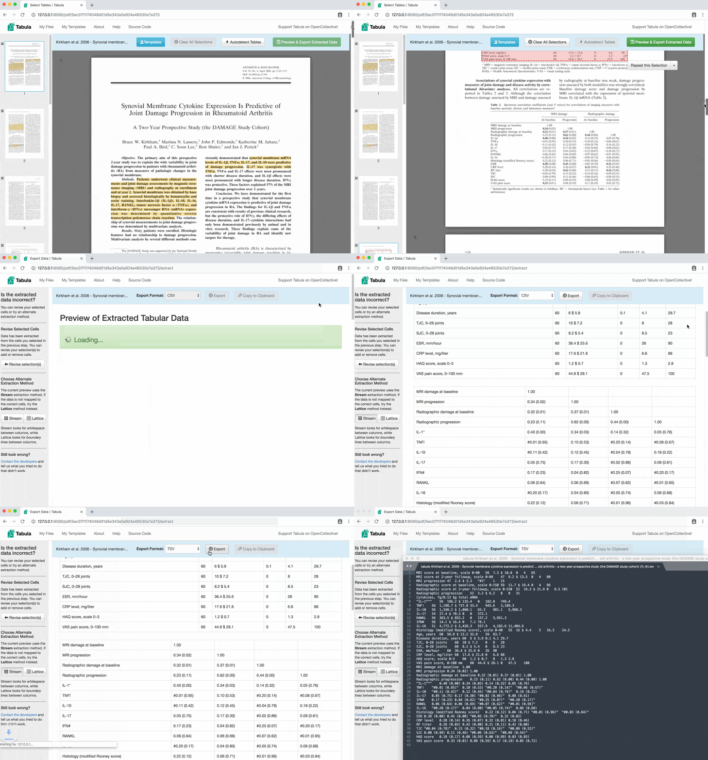 #'
#' # Download Tabula
#'
#' Go to tabula.technology and download the
#' version for your operating system.
#'
#'
#'
#' # Download Tabula
#'
#' Go to tabula.technology and download the
#' version for your operating system.
#'
#'  #'
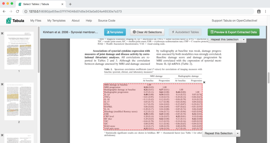
#' # Mark each table with your mouse
#'
#' When you launch Tabula, you will see a new web site hosted at `127.0.0.1:8080`.
#' Open a PDF file to get started. With your mouse, click and drag to make a
#' selection over each table in the PDF file. Don't include extra things like
#' headers or notes below the table, because they usually won't be recognized
#' correctly.
#'
#'
#'
#' # Mark each table with your mouse
#'
#' When you launch Tabula, you will see a new web site hosted at `127.0.0.1:8080`.
#' Open a PDF file to get started. With your mouse, click and drag to make a
#' selection over each table in the PDF file. Don't include extra things like
#' headers or notes below the table, because they usually won't be recognized
#' correctly.
#'
#'  #'
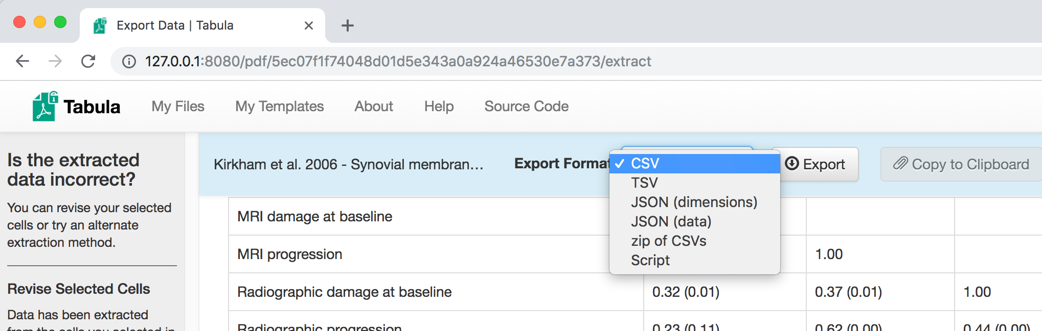
#' # Export the data as a CSV or script
#'
#' You can export the data as a comma-separated-values (CSV) file,
#' tab-separated-values (TSV) file, JSON, a zip file with multiple CSV files, or
#' even as a shell script you can run from the command line.
#'
#'
#'
#' # Export the data as a CSV or script
#'
#' You can export the data as a comma-separated-values (CSV) file,
#' tab-separated-values (TSV) file, JSON, a zip file with multiple CSV files, or
#' even as a shell script you can run from the command line.
#'
#'  #'
#' For example, here is the shell script that I got by selecting `Script` as the
#' export format:
#'
#' ```bash
#' java -jar tabula-java.jar -a 118.958,100.598,327.803,510.638 -p 4 "$1"
#' ```
#'
#' With this script, we don't need to launch the Tabula app. We can run the jar
#' file from the command line, giving the coordinates of the table with `-a` and
#' the page number with `-p`. The `"$1"` argument represents the name of the PDF
#' file.
#'
#' See [tabula-java](https://github.com/tabulapdf/tabula-java) for more details
#' about the Java command line application.
#'
#' # :floppy_disk: Download the data and code
#'
#' We can use [RStudio] to clean up the exported data with Find and Replace. Then,
#' we can use R and [ggplot2] to visualize the data.
#'
#' [RStudio]: https://www.rstudio.com/
#' [ggplot2]: https://ggplot2.tidyverse.org/
#'
#' Download the code for the figures here:
#'
#' - Kirkham2006.R
#'
#' Here is the data, cleaned up and ready for making figures:
#'
#'
#'
#' Below, you can see the figures I created for Tables 1, 2, and 3.
#'
#' # Figures
#'
#' ## Figure for Table 1
#'
#'
## ----table1, warning = FALSE, fig.height = 4, fig.width = 5.25, echo = FALSE, dpi = 300----
# Cytokines, fg/0.13 $g total mRNA
t1 <- read_tsv(col_names = FALSE,
file = "MRI score at baseline, scale 0–80 58 7.3 10.8 0 4 65
MRI score at 2-year followup, scale 0–80 47 9.2 13.5 0 4 80
MRI progression 47 2.4 3.3 1 1 15
Radiographic score at baseline, scale 0–150 59 11.7 19.4 0 4 96
Radiographic score at 2-year followup, scale 0–150 52 16.3 21.9 0 8.5 101
Radiographic progression 52 3.2 6.2 0 0 31
IL-1 56 196.2 135.4 0 182.8 749.4
TNFa 56 1,198.7 737.8 33.4 945.6 3,189.3
IL-10 56 1,348.2 1,060.1 65.3 981.1 5,988.3
IL-17 54 27.4 70.3 0 0 372.1
RANKL 56 363.5 852.2 0 157.2 5,951.3
IFNg 56 14.1 16.4 0 7.1 78.1
IL-16 51 4,772.2 2,428.3 557.9 4,182.6 11,404.6
Histology (modified Rooney score), scale 0–40 55 16 4.4 5 16.3 24.3
Age, years 60 58.8 13.2 32.8 59 83.7
Disease duration, years 60 6 5.9 0.1 4.1 29.7
TJC, 0–28 joints 60 10 7.2 0 8 28
SJC, 0–28 joints 60 8.2 5.4 0 8.5 23
ESR, mm/hour 60 36.4 25.6 0 26 90
CRP level, mg/liter 60 17.6 21.8 0 6.6 88
HAQ score, scale 0–3 60 1.2 0.7 0 1.3 2.8
VAS pain score, 0–100 mm 60 44.8 28.1 0 47.5 100
")
x <- apply(
X = stringr::str_split_fixed(
string = stringr::str_replace_all(t1$X3, ",", ""),
pattern = " ",
n = 2
),
MARGIN = 2,
FUN = as.numeric
)
t1$mean <- x[,1]
t1$sd <- x[,2]
t1$X3 <- NULL
colnames(t1) <- c("item", "n_subjects", "min", "median", "max", "mean", "sd")
readr::write_tsv(t1, "data/Kirkham2006-Table1.tsv")
ggplot(t1[7:13,]) +
aes(
x = item,
y = mean,
ymin = sapply(mean - sd, function(x) max(1, x)),
ymax = mean + sd
) +
geom_hline(
yintercept = as.vector(sapply(10^c(0:3), function(i) i * 1:10)),
size = 0.25,
color = "grey90"
) +
geom_errorbar(width = 0, size = 0.25) +
geom_point(size = 3) +
coord_flip() +
theme_bw(base_size = 20) +
annotate(
geom = "rect",
xmin = seq(1, 7, by = 2) - 0.5,
xmax = seq(1, 7, by = 2) + 0.5,
ymin = 0,
ymax = Inf,
alpha = 0.1
) +
scale_y_log10(
labels = scales::comma,
limits = c(1, 10000),
breaks = 10^c(0:4)
) +
labs(
title = "Laboratory findings in patients\nwith rheumatoid arthritis (n ≥ 51)",
x = NULL, y = "Cytokines, fg/0.13 μg total mRNA",
caption = "Data from Table 1, Kirkham et al. 2006. DOI: 10.1002/art.21749"
) +
theme(
title = element_text(size = 14),
panel.grid = element_blank(),
axis.ticks.y = element_blank()
)
#'
#'
#' ## Figure for Table 2
#'
#'
## ----table2, warning = FALSE, fig.width = 8, fig.height = 7, fig.retina = TRUE, echo = FALSE, dpi = 300----
t2 <- read_tsv(
col_names = FALSE,
file = "MRI damage at baseline 1.00
MRI progression 0.34 (0.02) 1.00
Radiographic damage at baseline 0.32 (0.01) 0.37 (0.01) 1.00
Radiographic progression 0.23 (0.11) 0.62 (0.00) 0.44 (0.00) 1.00
IL-1B 0.40 (0.00) 0.34 (0.03) 0.14 (0.32) 0.05 (0.76)
TNFa -0.01 (0.95) 0.10 (0.53) -0.20 (0.14) -0.06 (0.67)
IL-10 -0.11 (0.42) 0.12 (0.45) -0.04 (0.79) 0.18 (0.22)
IL-17 0.05 (0.75) 0.17 (0.30) -0.02 (0.86) 0.08 (0.61)
IFNg 0.17 (0.23) 0.04 (0.82) -0.25 (0.07) -0.20 (0.17)
RANKL 0.06 (0.64) 0.06 (0.69) -0.07 (0.62) -0.01 (0.95)
IL-16 -0.20 (0.17) 0.04 (0.80) -0.05 (0.74) 0.06 (0.68)
Histology (modified Rooney score) 0.22 (0.12) 0.06 (0.71) -0.01 (0.96) -0.03 (0.84)
ESR 0.38 (0.00) 0.45 (0.00) -0.05 (0.70) 0.32 (0.02)
CRP level 0.20 (0.14) 0.26 (0.07) 0.32 (0.01) 0.10 (0.46)
RF titer 0.28 (0.03) 0.42 (0.00) 0.21 (0.11) 0.42 (0.00)
TJC -0.04 (0.78) 0.15 (0.32) -0.18 (0.16) -0.09 (0.52)
SJC 0.00 (0.99) 0.11 (0.46) -0.06 (0.63) -0.09 (0.54)
HAQ score 0.18 (0.17) 0.08 (0.59) 0.00 (0.99) 0.03 (0.85)
VAS pain score 0.33 (0.01) 0.08 (0.59) 0.17 (0.19) 0.05 (0.72)
")
get_col <- function(t2, col) {
mri_baseline <- as.data.frame(
apply(
str_split_fixed(
str_replace_all(t2[[col]], "[()]", ""), " ", 2),
2, as.numeric
)
)
colnames(mri_baseline) <- c("spearman", "pvalue")
rownames(mri_baseline) <- t2$X1
mri_baseline <- mri_baseline[2:nrow(mri_baseline),]
mri_baseline$item <- rownames(mri_baseline)
mri_baseline
}
mri_baseline <- get_col(t2, 2)
p1 <- ggplot(mri_baseline) +
aes(
x = reorder(item, pvalue),
y = spearman,
fill = pvalue < 0.05 / nrow(mri_baseline)
) +
geom_hline(yintercept = 0, size = 0.25) +
geom_point(size = 3, shape = 21) +
coord_flip() +
theme_bw(base_size = 20) +
scale_fill_manual(values = c("white", "black"), guide = FALSE) +
annotate(
geom = "rect",
xmin = seq(1, 18, by = 2) - 0.5,
xmax = seq(1, 18, by = 2) + 0.5,
ymin = -Inf,
ymax = Inf,
alpha = 0.1
) +
labs(
x = NULL,
y = "Spearman",
title = "Correlation with MRI damage\nat baseline",
caption = "Data from Kirkham et al. 2006. DOI: 10.1002/art.21749"
) +
theme(
title = element_text(size = 14),
axis.ticks.x = element_line(size = 0.5),
panel.grid = element_blank(), axis.ticks.y = element_blank()
)
d2 <- rbind(
cbind(get_col(t2, 2), type = "MRI_Baseline"),
cbind(get_col(t2, 3), type = "MRI_Progression"),
cbind(get_col(t2, 4), type = "Radio_Baseline"),
cbind(get_col(t2, 5), type = "Radio_Progression")
)
rownames(d2) <- seq(nrow(d2))
m2 <- data.table::dcast(d2, item ~ type, value.var = "spearman")
m2_rows <- m2$item
m2 <- as.matrix(m2[,2:ncol(m2)])
rownames(m2) <- m2_rows
readr::write_tsv(d2, "data/Kirkham2006-Table2.tsv")
ggplot(d2) +
aes(y = item, x = type, fill = spearman) +
geom_tile(size = 0.5, color = "white") +
geom_text(aes(label = ifelse(pvalue < 0.05 / nrow(d2), spearman, "")), size = 5) +
# geom_point(color = ifelse(d2$pvalue < 0.05 / nrow(d2), "white", NA), size = 3) +
scale_size_manual(values = c(0, 1)) +
scale_fill_distiller(palette = "RdBu", limits = c(-1, 1)) +
theme_bw(base_size = 20) +
labs(
x = NULL,
y = NULL,
title = NULL,
caption = "Data from Table 2, Kirkham et al. 2006. DOI: 10.1002/art.21749"
) +
guides(
fill = guide_colorbar(
title.theme = element_text(size = 18),
ticks.colour = "black",
frame.linewidth = 1,
frame.colour = "black",
barwidth = 1,
barheight = 15,
title = "Spearman"
)
) +
scale_x_discrete(expand = c(0, 0), position = "top") +
scale_y_discrete(expand = c(0, 0)) +
theme(
title = element_text(size = 14),
axis.ticks.y = element_line(size = 0.5),
axis.ticks.x = element_line(size = 0.5),
axis.text.x = element_text(angle = 30, hjust = 0),
panel.grid = element_blank()
)
#'
#'
#' ## Figure for Table 3
#'
#'
## ----table3, warning = FALSE, fig.width = 9, fig.height = 6, fig.retina = TRUE, echo = FALSE, dpi = 300----
# Spearman correlation coefficients (and P values) for correlations of baseline
# synovial cytokine and histology measures with clinical and laboratory measures
t3 <- read_tsv(
col_names = FALSE,
file = "IL-1B 1.00
TNFa 0.22 (0.11) 1.00
IL-10 0.07 (0.63) 0.42 (0.000) 1.00
IL-17 0.40 (0.00) 0.21 (0.13) 0.29 (0.030) 1.00
RANKL -0.03 (0.81) 0.10 (0.47) 0.05 (0.71) 0.23 (0.09) 1.00
IFNg 0.67 (0.00) 0.42 (0.00) 0.24 (0.07) 0.52 (0.00) 0.11 (0.41) 1.00
IL-16 -0.02 (0.88) 0.29 (0.04) 0.32 (0.02) 0.45 (0.00) 0.23 (0.10) 0.09 (0.53) 1.00
Histology (modified Rooney score) 0.58 (0.00) -0.11 (0.44) -0.07 (0.67) 0.40 (0.00) -0.11 (0.44) 0.52 (0.00) 0.00 (0.98)
RF titer 0.03 (0.81) 0.11 (0.41) -0.01 (0.97) -0.07 (0.63) 0.01 (0.93) -0.17 (0.20) 0.00 (0.98)
ESR 0.46 (0.00) -0.03 (0.81) 0.02 (0.89) 0.38 (0.00) -0.04 (0.78) 0.35 (0.01) 0.01 (0.92)
CRP level 0.39 (0.00) -0.08 (0.54) -0.02 (0.87) 0.52 (0.00) 0.00 (0.98) 0.19 (0.15) 0.16 (0.26)
TJC -0.09 (0.51) 0.11 (0.43) 0.08 (0.58) 0.06 (0.66) 0.28 (0.04) 0.19 (0.15) 0.16 (0.26)
SJC 0.03 (0.83) 0.32 (0.02) 0.19 (0.16) -0.01 (0.96) 0.21 (0.12) 0.08 (0.54) 0.01 (0.95)
HAQ score 0.30 (0.03) 0.05 (0.69) $0.32 (0.01) 0.13 (0.36) -0.14 (0.29) 0.26 (0.05) -0.14 (0.34)
VAS pain score 0.02 (0.90) -0.01 (0.96) -0.24 (0.07) -0.08 (0.59) -0.01 (0.92) 0.01 (0.94) 0.03 (0.82)
")
t3_sm <- as.matrix(t3[,2:ncol(t3)])
t3_sm <- apply(t3_sm, 2, function(i) as.numeric(str_split_fixed(i, " ", 2)[,1]))
rownames(t3_sm) <- t3$X1
colnames(t3_sm) <- rownames(t3_sm)[1:7]
t3_sm <- t(t3_sm)
t3_sm[is.na(t3_sm)] <- 0
t3_pm <- as.matrix(t3[,2:ncol(t3)])
t3_pm <- apply(t3_pm, 2, function(i) {
as.numeric(str_split_fixed(str_replace_all(i, "[()]", ""), " ", 2)[,2])
})
rownames(t3_pm) <- t3$X1
colnames(t3_pm) <- rownames(t3_pm)[1:7]
t3_pm <- t(t3_pm)
t3_pm[is.na(t3_pm)] <- 0
o <- seriate(t3_sm)
t3_sm <- t3_sm[o[[1]], o[[2]]]
t3_pm <- t3_pm[o[[1]], o[[2]]]
t3_sm <- t3_sm %>% reshape2::melt() %>% filter(!is.na(value))
t3_pm <- t3_pm %>% reshape2::melt() %>% filter(!is.na(value))
colnames(t3_sm) <- c("var1", "var2", "spearman")
readr::write_tsv(t3_sm, "data/Kirkham2006-Table3.tsv")
ggplot(t3_sm) +
aes(x = var1, y = var2, fill = spearman) +
geom_tile(color = "white", size = 0.5) +
scale_fill_distiller(palette = "RdBu", limits = c(-1, 1)) +
theme_bw(base_size = 20) +
labs(
x = NULL,
y = NULL,
title = NULL,
caption = "Data from Table 3, Kirkham et al. 2006. DOI: 10.1002/art.21749"
) +
guides(
fill = guide_colorbar(
title.theme = element_text(size = 18),
ticks.colour = "black",
frame.linewidth = 1,
frame.colour = "black",
barwidth = 1,
barheight = 15,
title = "Spearman"
)
) +
scale_x_discrete(expand = c(0, 0), position = "top") +
scale_y_discrete(expand = c(0, 0)) +
theme(
axis.text.x = element_text(angle = 30, hjust = 0),
title = element_text(size = 14),
axis.ticks.x = element_line(size = 0.5),
axis.ticks.y = element_line(size = 0.5),
panel.grid = element_blank()
)
#'
#'
#'
#' For example, here is the shell script that I got by selecting `Script` as the
#' export format:
#'
#' ```bash
#' java -jar tabula-java.jar -a 118.958,100.598,327.803,510.638 -p 4 "$1"
#' ```
#'
#' With this script, we don't need to launch the Tabula app. We can run the jar
#' file from the command line, giving the coordinates of the table with `-a` and
#' the page number with `-p`. The `"$1"` argument represents the name of the PDF
#' file.
#'
#' See [tabula-java](https://github.com/tabulapdf/tabula-java) for more details
#' about the Java command line application.
#'
#' # :floppy_disk: Download the data and code
#'
#' We can use [RStudio] to clean up the exported data with Find and Replace. Then,
#' we can use R and [ggplot2] to visualize the data.
#'
#' [RStudio]: https://www.rstudio.com/
#' [ggplot2]: https://ggplot2.tidyverse.org/
#'
#' Download the code for the figures here:
#'
#' - Kirkham2006.R
#'
#' Here is the data, cleaned up and ready for making figures:
#'
#'
#'
#' Below, you can see the figures I created for Tables 1, 2, and 3.
#'
#' # Figures
#'
#' ## Figure for Table 1
#'
#'
## ----table1, warning = FALSE, fig.height = 4, fig.width = 5.25, echo = FALSE, dpi = 300----
# Cytokines, fg/0.13 $g total mRNA
t1 <- read_tsv(col_names = FALSE,
file = "MRI score at baseline, scale 0–80 58 7.3 10.8 0 4 65
MRI score at 2-year followup, scale 0–80 47 9.2 13.5 0 4 80
MRI progression 47 2.4 3.3 1 1 15
Radiographic score at baseline, scale 0–150 59 11.7 19.4 0 4 96
Radiographic score at 2-year followup, scale 0–150 52 16.3 21.9 0 8.5 101
Radiographic progression 52 3.2 6.2 0 0 31
IL-1 56 196.2 135.4 0 182.8 749.4
TNFa 56 1,198.7 737.8 33.4 945.6 3,189.3
IL-10 56 1,348.2 1,060.1 65.3 981.1 5,988.3
IL-17 54 27.4 70.3 0 0 372.1
RANKL 56 363.5 852.2 0 157.2 5,951.3
IFNg 56 14.1 16.4 0 7.1 78.1
IL-16 51 4,772.2 2,428.3 557.9 4,182.6 11,404.6
Histology (modified Rooney score), scale 0–40 55 16 4.4 5 16.3 24.3
Age, years 60 58.8 13.2 32.8 59 83.7
Disease duration, years 60 6 5.9 0.1 4.1 29.7
TJC, 0–28 joints 60 10 7.2 0 8 28
SJC, 0–28 joints 60 8.2 5.4 0 8.5 23
ESR, mm/hour 60 36.4 25.6 0 26 90
CRP level, mg/liter 60 17.6 21.8 0 6.6 88
HAQ score, scale 0–3 60 1.2 0.7 0 1.3 2.8
VAS pain score, 0–100 mm 60 44.8 28.1 0 47.5 100
")
x <- apply(
X = stringr::str_split_fixed(
string = stringr::str_replace_all(t1$X3, ",", ""),
pattern = " ",
n = 2
),
MARGIN = 2,
FUN = as.numeric
)
t1$mean <- x[,1]
t1$sd <- x[,2]
t1$X3 <- NULL
colnames(t1) <- c("item", "n_subjects", "min", "median", "max", "mean", "sd")
readr::write_tsv(t1, "data/Kirkham2006-Table1.tsv")
ggplot(t1[7:13,]) +
aes(
x = item,
y = mean,
ymin = sapply(mean - sd, function(x) max(1, x)),
ymax = mean + sd
) +
geom_hline(
yintercept = as.vector(sapply(10^c(0:3), function(i) i * 1:10)),
size = 0.25,
color = "grey90"
) +
geom_errorbar(width = 0, size = 0.25) +
geom_point(size = 3) +
coord_flip() +
theme_bw(base_size = 20) +
annotate(
geom = "rect",
xmin = seq(1, 7, by = 2) - 0.5,
xmax = seq(1, 7, by = 2) + 0.5,
ymin = 0,
ymax = Inf,
alpha = 0.1
) +
scale_y_log10(
labels = scales::comma,
limits = c(1, 10000),
breaks = 10^c(0:4)
) +
labs(
title = "Laboratory findings in patients\nwith rheumatoid arthritis (n ≥ 51)",
x = NULL, y = "Cytokines, fg/0.13 μg total mRNA",
caption = "Data from Table 1, Kirkham et al. 2006. DOI: 10.1002/art.21749"
) +
theme(
title = element_text(size = 14),
panel.grid = element_blank(),
axis.ticks.y = element_blank()
)
#'
#'
#' ## Figure for Table 2
#'
#'
## ----table2, warning = FALSE, fig.width = 8, fig.height = 7, fig.retina = TRUE, echo = FALSE, dpi = 300----
t2 <- read_tsv(
col_names = FALSE,
file = "MRI damage at baseline 1.00
MRI progression 0.34 (0.02) 1.00
Radiographic damage at baseline 0.32 (0.01) 0.37 (0.01) 1.00
Radiographic progression 0.23 (0.11) 0.62 (0.00) 0.44 (0.00) 1.00
IL-1B 0.40 (0.00) 0.34 (0.03) 0.14 (0.32) 0.05 (0.76)
TNFa -0.01 (0.95) 0.10 (0.53) -0.20 (0.14) -0.06 (0.67)
IL-10 -0.11 (0.42) 0.12 (0.45) -0.04 (0.79) 0.18 (0.22)
IL-17 0.05 (0.75) 0.17 (0.30) -0.02 (0.86) 0.08 (0.61)
IFNg 0.17 (0.23) 0.04 (0.82) -0.25 (0.07) -0.20 (0.17)
RANKL 0.06 (0.64) 0.06 (0.69) -0.07 (0.62) -0.01 (0.95)
IL-16 -0.20 (0.17) 0.04 (0.80) -0.05 (0.74) 0.06 (0.68)
Histology (modified Rooney score) 0.22 (0.12) 0.06 (0.71) -0.01 (0.96) -0.03 (0.84)
ESR 0.38 (0.00) 0.45 (0.00) -0.05 (0.70) 0.32 (0.02)
CRP level 0.20 (0.14) 0.26 (0.07) 0.32 (0.01) 0.10 (0.46)
RF titer 0.28 (0.03) 0.42 (0.00) 0.21 (0.11) 0.42 (0.00)
TJC -0.04 (0.78) 0.15 (0.32) -0.18 (0.16) -0.09 (0.52)
SJC 0.00 (0.99) 0.11 (0.46) -0.06 (0.63) -0.09 (0.54)
HAQ score 0.18 (0.17) 0.08 (0.59) 0.00 (0.99) 0.03 (0.85)
VAS pain score 0.33 (0.01) 0.08 (0.59) 0.17 (0.19) 0.05 (0.72)
")
get_col <- function(t2, col) {
mri_baseline <- as.data.frame(
apply(
str_split_fixed(
str_replace_all(t2[[col]], "[()]", ""), " ", 2),
2, as.numeric
)
)
colnames(mri_baseline) <- c("spearman", "pvalue")
rownames(mri_baseline) <- t2$X1
mri_baseline <- mri_baseline[2:nrow(mri_baseline),]
mri_baseline$item <- rownames(mri_baseline)
mri_baseline
}
mri_baseline <- get_col(t2, 2)
p1 <- ggplot(mri_baseline) +
aes(
x = reorder(item, pvalue),
y = spearman,
fill = pvalue < 0.05 / nrow(mri_baseline)
) +
geom_hline(yintercept = 0, size = 0.25) +
geom_point(size = 3, shape = 21) +
coord_flip() +
theme_bw(base_size = 20) +
scale_fill_manual(values = c("white", "black"), guide = FALSE) +
annotate(
geom = "rect",
xmin = seq(1, 18, by = 2) - 0.5,
xmax = seq(1, 18, by = 2) + 0.5,
ymin = -Inf,
ymax = Inf,
alpha = 0.1
) +
labs(
x = NULL,
y = "Spearman",
title = "Correlation with MRI damage\nat baseline",
caption = "Data from Kirkham et al. 2006. DOI: 10.1002/art.21749"
) +
theme(
title = element_text(size = 14),
axis.ticks.x = element_line(size = 0.5),
panel.grid = element_blank(), axis.ticks.y = element_blank()
)
d2 <- rbind(
cbind(get_col(t2, 2), type = "MRI_Baseline"),
cbind(get_col(t2, 3), type = "MRI_Progression"),
cbind(get_col(t2, 4), type = "Radio_Baseline"),
cbind(get_col(t2, 5), type = "Radio_Progression")
)
rownames(d2) <- seq(nrow(d2))
m2 <- data.table::dcast(d2, item ~ type, value.var = "spearman")
m2_rows <- m2$item
m2 <- as.matrix(m2[,2:ncol(m2)])
rownames(m2) <- m2_rows
readr::write_tsv(d2, "data/Kirkham2006-Table2.tsv")
ggplot(d2) +
aes(y = item, x = type, fill = spearman) +
geom_tile(size = 0.5, color = "white") +
geom_text(aes(label = ifelse(pvalue < 0.05 / nrow(d2), spearman, "")), size = 5) +
# geom_point(color = ifelse(d2$pvalue < 0.05 / nrow(d2), "white", NA), size = 3) +
scale_size_manual(values = c(0, 1)) +
scale_fill_distiller(palette = "RdBu", limits = c(-1, 1)) +
theme_bw(base_size = 20) +
labs(
x = NULL,
y = NULL,
title = NULL,
caption = "Data from Table 2, Kirkham et al. 2006. DOI: 10.1002/art.21749"
) +
guides(
fill = guide_colorbar(
title.theme = element_text(size = 18),
ticks.colour = "black",
frame.linewidth = 1,
frame.colour = "black",
barwidth = 1,
barheight = 15,
title = "Spearman"
)
) +
scale_x_discrete(expand = c(0, 0), position = "top") +
scale_y_discrete(expand = c(0, 0)) +
theme(
title = element_text(size = 14),
axis.ticks.y = element_line(size = 0.5),
axis.ticks.x = element_line(size = 0.5),
axis.text.x = element_text(angle = 30, hjust = 0),
panel.grid = element_blank()
)
#'
#'
#' ## Figure for Table 3
#'
#'
## ----table3, warning = FALSE, fig.width = 9, fig.height = 6, fig.retina = TRUE, echo = FALSE, dpi = 300----
# Spearman correlation coefficients (and P values) for correlations of baseline
# synovial cytokine and histology measures with clinical and laboratory measures
t3 <- read_tsv(
col_names = FALSE,
file = "IL-1B 1.00
TNFa 0.22 (0.11) 1.00
IL-10 0.07 (0.63) 0.42 (0.000) 1.00
IL-17 0.40 (0.00) 0.21 (0.13) 0.29 (0.030) 1.00
RANKL -0.03 (0.81) 0.10 (0.47) 0.05 (0.71) 0.23 (0.09) 1.00
IFNg 0.67 (0.00) 0.42 (0.00) 0.24 (0.07) 0.52 (0.00) 0.11 (0.41) 1.00
IL-16 -0.02 (0.88) 0.29 (0.04) 0.32 (0.02) 0.45 (0.00) 0.23 (0.10) 0.09 (0.53) 1.00
Histology (modified Rooney score) 0.58 (0.00) -0.11 (0.44) -0.07 (0.67) 0.40 (0.00) -0.11 (0.44) 0.52 (0.00) 0.00 (0.98)
RF titer 0.03 (0.81) 0.11 (0.41) -0.01 (0.97) -0.07 (0.63) 0.01 (0.93) -0.17 (0.20) 0.00 (0.98)
ESR 0.46 (0.00) -0.03 (0.81) 0.02 (0.89) 0.38 (0.00) -0.04 (0.78) 0.35 (0.01) 0.01 (0.92)
CRP level 0.39 (0.00) -0.08 (0.54) -0.02 (0.87) 0.52 (0.00) 0.00 (0.98) 0.19 (0.15) 0.16 (0.26)
TJC -0.09 (0.51) 0.11 (0.43) 0.08 (0.58) 0.06 (0.66) 0.28 (0.04) 0.19 (0.15) 0.16 (0.26)
SJC 0.03 (0.83) 0.32 (0.02) 0.19 (0.16) -0.01 (0.96) 0.21 (0.12) 0.08 (0.54) 0.01 (0.95)
HAQ score 0.30 (0.03) 0.05 (0.69) $0.32 (0.01) 0.13 (0.36) -0.14 (0.29) 0.26 (0.05) -0.14 (0.34)
VAS pain score 0.02 (0.90) -0.01 (0.96) -0.24 (0.07) -0.08 (0.59) -0.01 (0.92) 0.01 (0.94) 0.03 (0.82)
")
t3_sm <- as.matrix(t3[,2:ncol(t3)])
t3_sm <- apply(t3_sm, 2, function(i) as.numeric(str_split_fixed(i, " ", 2)[,1]))
rownames(t3_sm) <- t3$X1
colnames(t3_sm) <- rownames(t3_sm)[1:7]
t3_sm <- t(t3_sm)
t3_sm[is.na(t3_sm)] <- 0
t3_pm <- as.matrix(t3[,2:ncol(t3)])
t3_pm <- apply(t3_pm, 2, function(i) {
as.numeric(str_split_fixed(str_replace_all(i, "[()]", ""), " ", 2)[,2])
})
rownames(t3_pm) <- t3$X1
colnames(t3_pm) <- rownames(t3_pm)[1:7]
t3_pm <- t(t3_pm)
t3_pm[is.na(t3_pm)] <- 0
o <- seriate(t3_sm)
t3_sm <- t3_sm[o[[1]], o[[2]]]
t3_pm <- t3_pm[o[[1]], o[[2]]]
t3_sm <- t3_sm %>% reshape2::melt() %>% filter(!is.na(value))
t3_pm <- t3_pm %>% reshape2::melt() %>% filter(!is.na(value))
colnames(t3_sm) <- c("var1", "var2", "spearman")
readr::write_tsv(t3_sm, "data/Kirkham2006-Table3.tsv")
ggplot(t3_sm) +
aes(x = var1, y = var2, fill = spearman) +
geom_tile(color = "white", size = 0.5) +
scale_fill_distiller(palette = "RdBu", limits = c(-1, 1)) +
theme_bw(base_size = 20) +
labs(
x = NULL,
y = NULL,
title = NULL,
caption = "Data from Table 3, Kirkham et al. 2006. DOI: 10.1002/art.21749"
) +
guides(
fill = guide_colorbar(
title.theme = element_text(size = 18),
ticks.colour = "black",
frame.linewidth = 1,
frame.colour = "black",
barwidth = 1,
barheight = 15,
title = "Spearman"
)
) +
scale_x_discrete(expand = c(0, 0), position = "top") +
scale_y_discrete(expand = c(0, 0)) +
theme(
axis.text.x = element_text(angle = 30, hjust = 0),
title = element_text(size = 14),
axis.ticks.x = element_line(size = 0.5),
axis.ticks.y = element_line(size = 0.5),
panel.grid = element_blank()
)
#'
#'