Working with a sparse matrix in R
Sparse matrices are necessary for dealing with large single-cell RNA-seq
datasets. They require less memory than dense matrices, and they allow some
computations to be more efficient. In this note, we’ll discuss the internals of
the dgCMatrix class with examples.
Install and load libraries#
Let’s get started by installing and loading the Matrix package, which provides the sparse matrix classes that we use in this note.
install.packages("Matrix")
library(Matrix)
Below, we’ll explore two Matrix formats and their corresponding classes:
- The triplet format in class
dgTMatrix - The compressed column format in class
dgCMatrix
The triplet format in dgTMatrix#
dgTMatrix is a class from the Matrix R package that implements:
general, numeric, sparse matrices in (a possibly redundant) triplet format
The format is easy to understand:
- Assume all unspecified entries in the matrix are equal to zero.
- Define the non-zero entries in triplet form
(i, j, x)where:iis the row numberjis the column numberxis the value
That’s all there is to it. Let’s make one:
m <- Matrix(nrow = 3, ncol = 6, data = 0, sparse = TRUE)
m <- as(m, "dgTMatrix") # by default, Matrix() returns dgCMatrix
m[1,2] <- 10
m[1,3] <- 20
m[3,4] <- 30
m
## 3 x 6 sparse Matrix of class "dgTMatrix"
##
## [1,] . 10 20  . . .
## [2,] .  .  .  . . .
## [3,] .  .  . 30 . .
And let’s see what is inside:
str(m)
## Formal class 'dgTMatrix' [package "Matrix"] with 6 slots
##   ..@ i       : int [1:3] 0 0 2
##   ..@ j       : int [1:3] 1 2 3
##   ..@ Dim     : int [1:2] 3 6
##   ..@ Dimnames:List of 2
##   .. ..$ : NULL
##   .. ..$ : NULL
##   ..@ x       : num [1:3] 10 20 30
##   ..@ factors : list()
The object has slots i, j, and x.
We can reconstruct the above sparse matrix like this:
d <- data.frame(
  i = m@i + 1,  # m@i is 0-based, not 1-based like everything else in R
  j = m@j + 1,  # m@j is 0-based, not 1-based like everything else in R
  x = m@x
)
d
##   i j  x
## 1 1 2 10
## 2 1 3 20
## 3 3 4 30
sparseMatrix(i = d$i, j = d$j, x = d$x, dims = c(3, 6))
## 3 x 6 sparse Matrix of class "dgCMatrix"
##
## [1,] . 10 20  . . .
## [2,] .  .  .  . . .
## [3,] .  .  . 30 . .
We can convert a sparse matrix to a data frame like this:
as.data.frame(summary(m))
##   i j  x
## 1 1 2 10
## 2 1 3 20
## 3 3 4 30
Since m@x gives us access to the data values, we can easily transform
the values with log2():
m@x <- log2(m@x + 1)
Matrix Market files use the triplet format#
Matrix Market files often end with the file extension .mtx.
Write a Matrix Market file:
writeMM(m, "matrix.mtx")
## NULL
Dump the contents of the file:
readLines("matrix.mtx")
## [1] "%%MatrixMarket matrix coordinate real general"
## [2] "3 6 3"
## [3] "1 2 3.4594316186372973"
## [4] "1 3 4.392317422778761"
## [5] "3 4 4.954196310386875"
This is the Matrix Market file format:
- The first line is a comment (starts with
%%). - The next line says there are 3 rows, 6 columns, and 3 non-zero values.
- The next 3 lines describe the values in triplet format
(i, j, x).
Read a Matrix Market file:
m <- readMM("matrix.mtx")
m
## 3 x 6 sparse Matrix of class "dgTMatrix"
##
## [1,] . 3.459432 4.392317 .        . .
## [2,] . .        .        .        . .
## [3,] . .        .        4.954196 . .
Convert from dgTMatrix to dgCMatrix with:
as(m, "dgCMatrix")
## 3 x 6 sparse Matrix of class "dgCMatrix"
##
## [1,] . 3.459432 4.392317 .        . .
## [2,] . .        .        .        . .
## [3,] . .        .        4.954196 . .
The compressed column format in dgCMatrix#
dgCMatrix is a class from the Matrix R package that implements:
general, numeric, sparse matrices in the (sorted) compressed sparse column format
This is the most common type of matrix that we will encounter when we are dealing with scRNA-seq data.
Let’s make a sparse matrix in the dgCMatrix format:
library(Matrix)
m <- Matrix(nrow = 3, ncol = 6, data = 0, sparse = TRUE)
m[1,2] <- 10
m[1,3] <- 20
m[3,4] <- 30
m
## 3 x 6 sparse Matrix of class "dgCMatrix"
##
## [1,] . 10 20  . . .
## [2,] .  .  .  . . .
## [3,] .  .  . 30 . .
Let’s look inside:
str(m)
## Formal class 'dgCMatrix' [package "Matrix"] with 6 slots
##   ..@ i       : int [1:3] 0 0 2
##   ..@ p       : int [1:7] 0 0 1 2 3 3 3
##   ..@ Dim     : int [1:2] 3 6
##   ..@ Dimnames:List of 2
##   .. ..$ : NULL
##   .. ..$ : NULL
##   ..@ x       : num [1:3] 10 20 30
##   ..@ factors : list()
The object has 6 slots, including Dim, i, x, and p.
Dim has dimensions of the matrix (3 rows, 6 columns):
m@Dim
## [1] 3 6
x has data values sorted column-wise (top to bottom, left to right):
m@x
## [1] 10 20 30
i has row indices for each data value. Note: i is 0-based, not 1-based
like everything else in R.
m@i
## [1] 0 0 2
What about p? Unlike j, p does not tell us which column each data value
us in.
m@p
## [1] 0 0 1 2 3 3 3
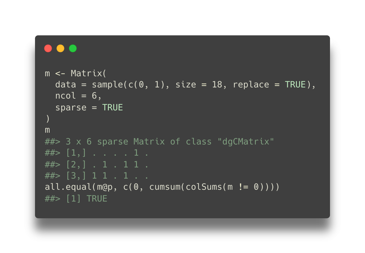
p has the cumulative number of data values as we move from one column
to the next column, left to right. The first value is always 0, and the
length of p is one more than the number of columns.
We can compute p for any matrix:
c(0, cumsum(colSums(m != 0)))
## [1] 0 0 1 2 3 3 3
Since p is a cumulative sum, we can use diff() to get the number of
non-zero entries in each column:
diff(m@p)
## [1] 0 1 1 1 0 0
colSums(m != 0)
## [1] 0 1 1 1 0 0
The length of p is one more than the number of columns:
length(m@p)
## [1] 7
m@Dim[2] + 1
## [1] 7
Given p, we can compute j:
rep(1:m@Dim[2], diff(m@p))
## [1] 2 3 4
Most of the time, it’s easier to use summary() to convert a sparse matrix to
triplet (i, j, x) format.
summary(m)$j
## [1] 2 3 4
One more example might help to clarify how i, x, and p change as we
modify the matrix:
# Add more values to the matrix
m[2,2] <- 50
m[2,3] <- 50
m[2,4] <- 50
m
## 3 x 6 sparse Matrix of class "dgCMatrix"
##
## [1,] . 10 20  . . .
## [2,] . 50 50 50 . .
## [3,] .  .  . 30 . .
str(m)
## Formal class 'dgCMatrix' [package "Matrix"] with 6 slots
##   ..@ i       : int [1:6] 0 1 0 1 1 2
##   ..@ p       : int [1:7] 0 0 2 4 6 6 6
##   ..@ Dim     : int [1:2] 3 6
##   ..@ Dimnames:List of 2
##   .. ..$ : NULL
##   .. ..$ : NULL
##   ..@ x       : num [1:6] 10 50 20 50 50 30
##   ..@ factors : list()
We know that p[1] is always 0.
Column 1 has 0 values, so p[2] is 0.
Column 2 has 2 values, so p[3] is 0 + 2 = 2.
Column 3 has 2 values, so p[4] is 2 + 2 = 4.
Column 4 has 2 values, so p[5] is 4 + 2 = 6.
Columns 5 and 6 have 0 values, so p[6] and p[7] are 6 + 0 = 6.
Here’s a visual representation of m@p for this example:

The vector p has the cumulative number of data values as we move from one
column to the next column, left to right.
Sparse matrices use less memory than dense matrices#
# A large matrix
set.seed(1)
m <- sparseMatrix(
  i = sample(x = 1e4, size = 1e4),
  j = sample(x = 1e4, size = 1e4),
  x = rnorm(n = 1e4)
)
pryr::object_size(m)
## 162 kB
pryr::object_size(as.matrix(m)) # Dense matrices require much more memory (RAM)
## 800 MB
Compute the sparsity of the matrix:
sparsity <- length(m@x) / m@Dim[1] / m@Dim[2]
sparsity
## [1] 1e-04
When writing Matrix Market files, remember to use gzip compression to save disk space.
writeMM(m, "matrix.mtx")
The uncompressed file size:
bytes_uncompressed <- file.size("matrix.mtx")
scales::number_bytes(bytes_uncompressed)
## [1] "281 KiB"
Compressing the file can save 50% of the disk space:
system("gzip --keep matrix.mtx")
file.size("matrix.mtx.gz") / bytes_uncompressed
## [1] 0.4883699
It takes about the same amount of time to read uncompressed or compressed Matrix Market files:
bench::mark(
  m <- readMM("matrix.mtx"),
  m <- readMM("matrix.mtx.gz")
)
## # A tibble: 2 x 6
##   expression                        min   median `itr/sec` mem_alloc `gc/sec`
##   <bch:expr>                   <bch:tm> <bch:tm>     <dbl> <bch:byt>    <dbl>
## 1 m <- readMM("matrix.mtx")      6.63ms   7.12ms      140.     626KB        0
## 2 m <- readMM("matrix.mtx.gz")   7.32ms   8.31ms      121.     626KB        0
writeMMgz#
Since the writeMM() function does not accept a connection object, this
does not work:
writeMM(m, gzfile("matrix.mtx.gz")) ## This does not work :(
Instead, we can write our own function:
#' @param x A sparse matrix from the Matrix package.
#' @param file A filename that ends in ".gz".
writeMMgz <- function(x, file) {
  mtype <- "real"
  if (is(x, "ngCMatrix")) {
    mtype <- "integer"
  }
  writeLines(
    c(
      sprintf("%%%%MatrixMarket matrix coordinate %s general", mtype),
      sprintf("%s %s %s", x@Dim[1], x@Dim[2], length(x@x))
    ),
    gzfile(file)
  )
  data.table::fwrite(
    x = summary(x),
    file = file,
    append = TRUE,
    sep = " ",
    row.names = FALSE,
    col.names = FALSE
  )
}
Confirm that it works:
writeMMgz(m, "matrix2.mtx.gz")

all.equal(readMM("matrix.mtx.gz"), readMM("matrix2.mtx.gz"))
## [1] TRUE
Some operations on sparse matrices are fast#
Let’s make a dense copy of the 10,000 by 10,000 sparse matrix.
d <- as.matrix(m)
Recall that only 10,000 (0.01%) of the entries in this matrices are non-zero.
Many operations are much faster on sparse matrices:
bench::mark(
  colSums(m),
  colSums(d)
)
## # A tibble: 2 x 6
##   expression      min   median `itr/sec` mem_alloc `gc/sec`
##   <bch:expr> <bch:tm> <bch:tm>     <dbl> <bch:byt>    <dbl>
## 1 colSums(m)  343.6µs  447.5µs    2194.      261KB        0
## 2 colSums(d)   91.9ms   92.6ms      10.6    78.2KB        0
bench::mark(
  rowSums(m),
  rowSums(d)
)
## # A tibble: 2 x 6
##   expression      min   median `itr/sec` mem_alloc `gc/sec`
##   <bch:expr> <bch:tm> <bch:tm>     <dbl> <bch:byt>    <dbl>
## 1 rowSums(m)    405µs    511µs   1973.     234.6KB     2.02
## 2 rowSums(d)    167ms    169ms      5.92    78.2KB     0
Suppose we want to collapse columns by summing groups of columns according to another variable.
set.seed(1)
y <- sample(1:10, size = ncol(m), replace = TRUE)
table(y)
## y
##    1    2    3    4    5    6    7    8    9   10
##  980  937  972 1018  974  979 1072 1023 1015 1030
Let’s turn the variable into a model matrix:
ymat <- model.matrix(~ 0 + factor(y))
colnames(ymat) <- 1:10
head(ymat)
##   1 2 3 4 5 6 7 8 9 10
## 1 0 0 0 0 0 0 0 0 1  0
## 2 0 0 0 1 0 0 0 0 0  0
## 3 0 0 0 0 0 0 1 0 0  0
## 4 1 0 0 0 0 0 0 0 0  0
## 5 0 1 0 0 0 0 0 0 0  0
## 6 0 0 0 0 0 0 1 0 0  0
colSums(ymat)
##    1    2    3    4    5    6    7    8    9   10
##  980  937  972 1018  974  979 1072 1023 1015 1030
And now we can collapse the columns that belong to each group:
x1 <- m %*% ymat
x2 <- d %*% ymat
all.equal(as.matrix(x1), x2)
## [1] TRUE
all.equal(x1[,1], rowSums(m[,y == 1]))
## [1] TRUE
all.equal(x1[,2], rowSums(m[,y == 2]))
## [1] TRUE
dim(x1)
## [1] 10000 10
head(x1)
## 6 x 10 Matrix of class "dgeMatrix"
##      1 2 3 4 5 6           7           8          9        10
## [1,] 0 0 0 0 0 0  0.00000000  0.00000000 -0.5578692 0.0000000
## [2,] 0 0 0 0 0 0  0.74277916  0.00000000  0.0000000 0.0000000
## [3,] 0 0 0 0 0 0  0.00000000  0.00000000  0.0000000 1.5986887
## [4,] 0 0 0 0 0 0  0.00000000  0.00000000  0.0000000 0.8402201
## [5,] 0 0 0 0 0 0  0.00000000 -0.09295838  0.0000000 0.0000000
## [6,] 0 0 0 0 0 0 -0.05341102  0.00000000  0.0000000 0.0000000
On my machine, this operation on this data is 100 times faster with a sparse matrix than with a dense matrix.
bench::mark(
  m %*% ymat,
  d %*% ymat,
  check = FALSE
)
## # A tibble: 2 x 6
##   expression      min   median `itr/sec` mem_alloc `gc/sec`
##   <bch:expr> <bch:tm> <bch:tm>     <dbl> <bch:byt>    <dbl>
## 1 m %*% ymat    603µs    844µs   1077.      1.75MB     4.18
## 2 d %*% ymat    838ms    838ms      1.19   781.3KB     0
R packages for working with sparse matrices#
You might consider trying these packages for working with sparse matrices in R:
- proxyC by Kohei Watanabe — R package for large-scale similarity/distance computation
- sparseMatrixStats by Constantin Ahlmann-Eltze — Implementation of the matrixStats API for sparse matrices
- RSpectra by Yixuan Qiu — R Interface to the Spectra Library for Large Scale Eigenvalue and SVD Problems
Learn more#
Find more details about additional matrix formats in this vignettes from the Matrix R package.
And learn more about faster computations with sparse matrices in this vignette.